Si/Ge (001) Valence Band Offset

1. Introduction

This tutorial calculates the valence band offset ΔE_v between germanium grown pseudomorphically on silicon (001) and silicon, reproducing the result of the following manuscript:

Manuscript

Chris G. Van de Walle and Richard M. Martin, "Theoretical calculations of heterojunction discontinuities in the Si/Ge system", Physical Review B 34, 5621 (1986). DOI:10.1103/PhysRevB.34.5621. ¹

This tutorial builds upon the Si/Ge (001) Strained Superlattice tutorial, where the superlattice and the two strained bulk cells are created. Here, the platform's valence band offset workflow runs Quantum ESPRESSO on all three, and the offset is assembled as in Sec. III.A of the manuscript: each bulk's valence band maximum E_VBM is measured from its own average potential V̄, and the superlattice gives the step in V̄ between the two materials,

ΔE_v = (E_VBM − V̄)_Ge − (E_VBM − V̄)_Si + (V̄_Ge − V̄_Si)_superlattice

The manuscript gives ΔE_v = 0.74 eV without spin–orbit coupling, Ge above Si (Sec. III.A), and 0.84 eV in Table I after adding 0.10 eV for the spin–orbit splitting of germanium by hand (Sec. IV).

2. Prerequisites

Before starting this tutorial, one of the following steps should be completed:

1. Follow the Si/Ge (001) Strained Superlattice tutorial, using the interface_3d_3d_silicon_germanium.ipynb notebook embedded in its section 6, to create and save Si/Ge (001) superlattice 4+4, Si (001) bulk a=5.43 and Ge (001) bulk a=5.43 c=5.82, OR
2. Have the three materials saved in the uploads folder or in the account's materials collection

3. Workflow overview

The calculation consists of the following steps:

1. Set up the environment and parameters: Configure the material names, the Density Functional Theory (DFT) model, and compute resources
2. Authenticate and initialize API client: Connect to the platform
3. Load materials: Import the superlattice and the two bulks, print their plane spacings
4. Configure the model and k-grids: One DFT model, a k-grid per material from one k-point density
5. Configure compute resources: Select the cluster, queue, and processor settings
6. Configure the workflow: The model, a k-grid per material, and the band structures the valence band maxima are read from
7. Run the job: One Valence Band Offset job, which runs a band structure and the electrostatic potential on each of the three materials
8. Retrieve results: The valence band maxima and average potentials, the offset, and the potential across the superlattice
9. Compare with the manuscript: Print our values beside Van de Walle & Martin's

4. Calculation parameters

	this tutorial	Van de Walle & Martin
Code	Quantum ESPRESSO	momentum-space pseudopotential code
Functional	local density approximation (LDA): Ceperley–Alder, Perdew–Zunger parametrization	the same
Pseudopotentials	ultrasoft, Garrity–Bennett–Rabe–Vanderbilt (GBRV) library, Ge 3d in valence	norm-conserving (Bachelet–Hamann–Schlüter)
Cutoff	40 / 200 Ry	6 Ry
k-points	5 points per Å⁻¹: 9×9×3 superlattice, 6×6×6 bulks	four special points
Cell	4 + 4 planes, 8 atoms, a∥ = 5.43, a_Ge⊥ = 5.82 Å	the same
Positions	ideal (Sec. II)	ideal
Reference potential V̄	planar average of the electrostatic potential	planar average of the l = 1 component of the total potential
Spin–orbit	not included	not included; +0.10 eV added for Table I

The two terms of the offset depend on the reference potential, so only their sum is compared with the manuscript (p. 5625). Both calculations are LDA: neither the offsets nor the Kohn–Sham gaps below are experimental values.

5. Step-by-step instructions

5.1. Open the notebook

Navigate to the API examples repository and open the notebook:

other/materials_designer/specific_examples/interface_3d_3d_silicon_germanium_SIMULATION.ipynb

5.2. Configure parameters

The parameters cells set the material names, the compute resources, and the DFT model:

SUPERLATTICE_NAME = "Si/Ge (001) superlattice 4+4"
SUBSTRATE_BULK_NAME = "Si (001) bulk a=5.43"
FILM_BULK_NAME = "Ge (001) bulk a=5.43 c=5.82"

CLUSTER_NAME = "001"
QUEUE_NAME = QueueName.OR
PPN = 16
TIME_LIMIT = "04:00:00"

MODEL_SUBTYPE = "lda"
FUNCTIONAL = "pz"
PSEUDOPOTENTIAL_TYPE = "us"
ECUTWFC = 40   # Ry
ECUTRHO = 200  # Ry
KPOINT_DENSITY = 5  # points per Å⁻¹

5.3. Run the notebook

Execute all cells by selecting Run > Run All from the menu.

The notebook first authenticates with the platform, then runs the steps listed in section 3.

5.4. Analyze results

Section 8.1 of the notebook prints each bulk's valence band maximum, its average potential and its gap, and the average potential of the Si and the Ge block in the superlattice:

Si (001) bulk a=5.43: E_VBM = 6.0108 eV, V̄ = 1.2535 eV, E_VBM - V̄ = 4.7573 eV, gap +0.474 eV
  in the superlattice: V̄ = 2.4459 eV, averaged over 1.3575 Å centred at z = 5.6250 Å
Ge (001) bulk a=5.43 c=5.82: E_VBM = 9.0797 eV, V̄ = 4.3315 eV, E_VBM - V̄ = 4.7482 eV, gap -0.088 eV
  in the superlattice: V̄ = 3.2203 eV, averaged over 1.4550 Å centred at z = 11.2500 Å

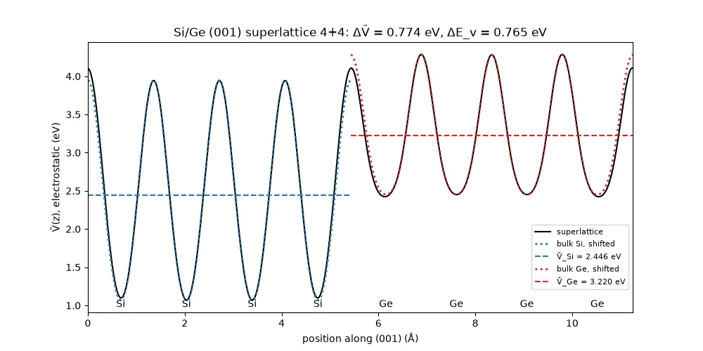
The valence band maximum is the top of band N_electrons / 2 along each bulk's k-path, and the gap the bottom of the next band minus it. The strained Ge is a semimetal in the LDA: its L conduction band lies 0.088 eV below the valence band top at Γ, hence the negative gap. Each block is averaged over one plane spacing at its centre, one plane away from both interfaces, where the manuscript finds the potential bulk-like (Fig. 2). Section 8.3 plots the potential across the superlattice with the bulk potentials overlaid, as in the manuscript's Fig. 2.

The last cell prints the offset beside the manuscript's values:

ΔE_v = 0.765 eV   paper 0.74 eV   deviation +3.4 %
ΔE_v + 0.10 eV = 0.865 eV   paper 0.84 eV   deviation +3.0 %
Ge valence band top above Si's   paper above
(E_VBM - V̄)_Ge - (E_VBM - V̄)_Si = -0.01 eV   paper -0.11 eV
(V̄_Ge - V̄_Si)_superlattice = +0.77 eV   paper +0.85 eV

6. Expected results

Sec. III.A of the manuscript gives ΔE_v = 0.74 eV for the (001) superlattice on silicon, Ge above Si, computed without spin–orbit coupling. Table I lists 0.84 eV for the same interface, after 0.10 eV is added for germanium's spin–orbit splitting (Sec. IV); this run is compared with both, the second after adding the same 0.10 eV. The manuscript's two terms, ΔV̄ = 0.85 eV and the bulk term 11.08 − 11.19 = −0.11 eV (p. 5625), are measured from the l = 1 component of the total potential, so they are printed for reference only: here the lineup is 0.08 eV smaller and the bulk term 0.10 eV larger than the manuscript's, and the sum is within 0.03 eV.

The manuscript compares with no experiment for this interface: the measured Si/Ge junctions were presumably not pseudomorphic (p. 5630). The band gaps printed in section 8.1 are Kohn–Sham gaps, smaller than the measured ones.

6.1. Comparison with published results

	ΔE_v (eV)	ΔE_v + 0.10 eV (eV)	bulk term (eV)	ΔV̄ (eV)
Van de Walle & Martin	0.74	0.84	−0.11 (l = 1 reference)	0.85 (l = 1 reference)
This tutorial	0.765 (+3.4 %)	0.865 (+3.0 %)	−0.009	0.774

The manuscript's Fig. 2 shows its potential across one period of the superlattice. The bulk potentials (dashed) coincide with it away from the interfaces, and their averages (dashed horizontal lines) are shifted with respect to each other:

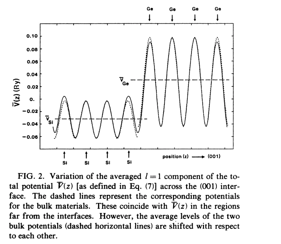
Section 8.3 of the notebook draws the same figure for this calculation: one period from the Ge→Si interface, each bulk's own potential (dotted) shifted onto its block, and the two averages (dashed). The bulk potentials coincide with the superlattice's inside both blocks and depart from it only at the interfaces, and the Ge average lies 0.77 eV above the Si one, against 0.85 eV in the manuscript. Here the atomic planes sit at the minima of the potential and its oscillation is larger in Si; in the manuscript's figure they sit at the maxima (the arrows) and the oscillation is larger in Ge. The curve plotted here is the electrostatic potential of these pseudopotentials, not the l = 1 component of the manuscript's total potential: its shape and the step between the two averages depend on that choice, ΔE_v does not (p. 5625).

7. Customization options

7.1. Adjust computational resources

CLUSTER_NAME selects the cluster by its full or partial name; a name that is not available makes the notebook stop and list the ones that are.

8. Troubleshooting

8.1. Material not found

If one of the three names is not found in the uploads folder or the account's materials collection, run the Si/Ge (001) Strained Superlattice tutorial first, and check that its uploads folder holds the materials under those exact names.

8.2. Offset far from the published value

Check the plane spacings printed in section 3 of the notebook first: 1.3575 Å in Si, 1.455 Å in Ge and 1.406 Å at both interfaces. Then check the gaps printed in section 8.1: about +0.47 eV for Si and −0.09 eV for Ge, whose L conduction band dips below the valence band top at Γ in the LDA. A different Ge gap means a different pseudopotential, cutoff or cell, and moves E_VBM of Ge and the offset with it.

9. Interactive JupyterLite notebook

The following JupyterLite notebook calculates the valence band offset. Select Run > Run All Cells.

⛶ Full Screen

10. References

---

1. Chris G. Van de Walle and Richard M. Martin. Theoretical calculations of heterojunction discontinuities in the Si/Ge system. Physical Review B, 34:5621–5634, 1986. URL: https://link.aps.org/doi/10.1103/PhysRevB.34.5621. ↩