Grain Boundary (2D) in h-BN (Band Gap and In-Gap States)

1. Introduction

This tutorial calculates the local density of states (LDOS) at the Type III 5|7 grain boundary of an h-BN monolayer and the density of states of the perfect layer, reproducing Fig. 4b of the following manuscript: the gap between the two LDOS peaks that border it, about 3.2 eV, the four boundary peaks, and the gap of the perfect layer.

Manuscript

Qiucheng Li, Xiaolong Zou, Mengxi Liu, Jingyu Sun, Yabo Gao, Yue Qi, Xiebo Zhou, Boris I. Yakobson, Yanfeng Zhang and Zhongfan Liu Grain Boundary Structures and Electronic Properties of Hexagonal Boron Nitride on Cu(111) Nano Letters 15 (9), 5804–5810 (2015) DOI: 10.1021/acs.nanolett.5b01852 ¹

2. Prerequisites

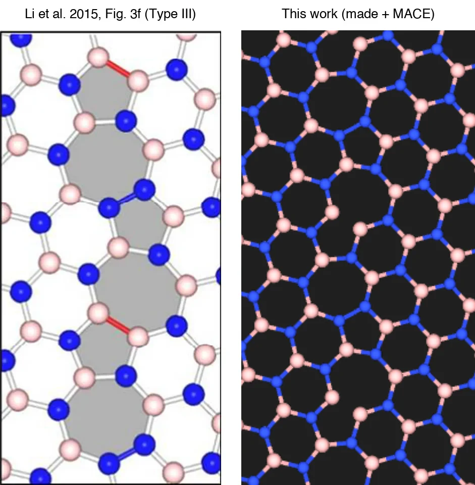
Run the structure notebook defect_planar_grain_boundary_2d_boron_nitride.ipynb first. It builds the (3,1)|(1,3) boundary at 32.2°, a cell of 208 atoms (62.7 × 9.05 Å) holding two boundaries, each a continuous 5-7-5-7 chain with one B–B and one N–N bond per period, relaxes it with MACE and saves it as h-BN 5-7 grain boundary, MACE-relaxed, the name this notebook loads.

3. Workflow overview

The notebook runs the Standata dos.json workflow once on the boundary cell and once on the perfect h-BN monolayer from Standata. It chains pw_scf, pw_nscf and projwfc, which writes the density of states projected on each atom.

The LDOS of the boundary is the sum over the atoms within BOUNDARY_DISTANCE of either boundary of the cell. The energy zero is the middle of the gap of the atoms farther than BULK_DISTANCE from both boundaries, as in Fig. 4b. With RELAX = True, a fixed-cell relaxation to 0.01 eV/Å runs first and the boundary job uses its final structure. A re-run finds each finished job by its material and workflow name and reuses it.

4. Calculation parameters

Cell 1.3 sets the relaxation switch and the compute:

from datetime import datetime
from mat3ra.ide.compute import QueueName

ORGANIZATION_NAME = None  # set to your organization name (full or partial); otherwise, your default one is used
FOLDER = "./uploads"

DOS_SEARCH_TERM = "dos.json"
RELAX_WORKFLOW_SEARCH_TERM = "fixed_cell_relaxation.json"
APPLICATION_NAME = "espresso"

# False: the MACE-relaxed boundary as saved. True: relax it with DFT to the manuscript's 0.01 eV/Å first, once.
RELAX = False

CLUSTER_NAME = "001"  # specify full or partial name i.e. "cluster-001" to select
QUEUE_NAME = QueueName.OR
PPN = 16  # OR allows 16 cores per job
TIME_LIMIT = "04:00:00"

timestamp = datetime.now().strftime("%Y-%m-%d %H:%M")
POLL_INTERVAL = 60  # seconds

Cell 1.4 sets the DFT parameters:

FUNCTIONAL = "pbe"  # the manuscript's functional (VASP, PAW)
PSEUDOPOTENTIAL_TYPE = "us"  # GBRV ultrasoft, the platform's default PBE family for B and N
ECUTWFC = 40  # Ry, GBRV's recommended wavefunction cutoff
ECUTRHO = 200  # Ry, GBRV's recommended charge-density cutoff

KPOINT_DENSITY = 4  # Å⁻¹, one density for both cells; the manuscript does not state its k-points
MODEL_TAG = f"{FUNCTIONAL}-{PSEUDOPOTENTIAL_TYPE} {ECUTWFC}-{ECUTRHO}Ry k{KPOINT_DENSITY}"

SCF_UNIT = "pw_scf"
NSCF_UNIT = "pw_nscf"
RELAX_UNIT = "pw_relax"
RELAXATION_SETTINGS = {"forc_conv_thr": 3.9e-4, "nstep": 100}  # 0.01 eV/Å, the manuscript's convergence target
# Names the relaxation job; the relaxed structure itself is found by content hash.
RELAX_TAG = f"{MODEL_TAG} f{RELAXATION_SETTINGS['forc_conv_thr']}"

Cell 1.5 sets how the LDOS is read:

BOUNDARY_DISTANCE = 2.0  # Å, atoms this close to a boundary make up its LDOS
BULK_DISTANCE = 5.0  # Å, atoms farther than this from both boundaries are the bulk, whose mid-gap is the energy zero
GAP_DOS_THRESHOLD = 0.02  # fraction of the maximum DOS below which an energy counts as inside the gap
PEAK_PROMINENCE = 0.1  # fraction of the maximum boundary LDOS in the window a peak must stand out by
ENERGY_WINDOW = (-4.0, 4.0)  # eV, the range of Fig. 4b

manuscript	this notebook
PBE	PBE
VASP, PAW; cutoff not stated	GBRV ultrasoft, 40/200 Ry
k-points not stated	4 Å⁻¹ for both cells: 1 × 3 × 1 for the boundary cell, 12 × 12 × 1 for the perfect layer
two antiparallel boundaries, cell about 6.5 nm across them	two antiparallel boundaries, cell 62.7 Å across them, 9.05 Å along
vacuum above 10 Å	vacuum 20 Å
DFT relaxation to 0.01 eV/Å	MACE relaxation to 0.01 eV/Å; DFT to 0.01 eV/Å with RELAX = True
LDOS projected on the boundary	sum of the per-atom densities of states within 2 Å of the boundaries

5. Step-by-step instructions

5.1. Open the notebook

Navigate to the API examples repository and open:

other/materials_designer/specific_examples/defect_planar_grain_boundary_2d_boron_nitride_SIMULATION.ipynb

5.2. Configure parameters

In cell 1.3, set ORGANIZATION_NAME to the account's organization. Cell 1.2 names the boundary as the structure notebook saves it and the perfect layer as Standata names it; cells 1.4 and 1.5 keep the defaults.

5.3. Run the notebook

Select Run > Run All. The notebook authenticates with the platform (section 2), loads the two materials, prints their composition and cell and saves them to the platform (section 3), configures one model and k-point density for both cells (section 4) and the compute (section 5), relaxes the boundary if RELAX (section 6), and creates and submits the two Density of States jobs (section 7). Section 8 reads the per-atom densities of states, the gap and the peaks, and plots the LDOS; section 9 prints the comparison with the manuscript.

5.4. Re-run the notebook

A re-run finds the finished jobs by material and workflow name and reuses them rather than resubmitting.

6. Expected results

The boundary is a continuous 5-7 chain with one B–B and one N–N bond per period, as in the manuscript.

The manuscript's values (the gap from the text, the peaks and the perfect layer's gap read off Fig. 4b) and the values measured by the notebook, with the MACE-relaxed boundary:

quantity	this work	Li et al. 2015
gap, peak (2) to peak (3)	3.20 eV	3.21 eV
peak (1)	−2.67 eV	−2.85 eV
peak (2)	−1.68 eV	−1.82 eV
peak (3)	+1.52 eV	+1.39 eV
peak (4)	+2.52 eV	+2.31 eV
perfect-layer gap	4.40 eV	4.4 eV

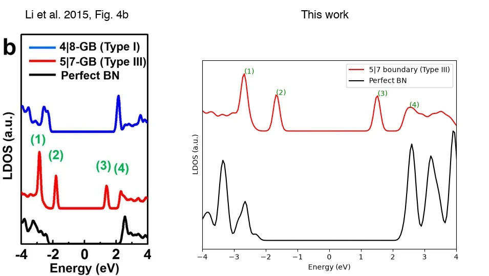
Peaks (2) and (3) lie inside the gap of the perfect layer and peaks (1) and (4) just outside it, in the manuscript and in this notebook.

7. Customization options

GRAIN_BOUNDARY_NAME selects the boundary; the commented alternative is the same cell as built, before the MACE relaxation. RELAX = True relaxes the boundary with DFT to the manuscript's 0.01 eV/Å before the Density of States job, and reuses a relaxed structure already on the account.

KPOINT_DENSITY, ECUTWFC and ECUTRHO set the k-point sampling and the plane-wave cutoffs. MODEL_TAG is built from these settings and is part of every workflow's name, so changing any of them creates new jobs rather than reusing the ones already run. The read-out parameters of cell 1.5 act on the finished jobs only.

8. Troubleshooting

8.1. Material not found

ValueError: No material named … means the structure notebook has not been run, or GRAIN_BOUNDARY_NAME does not match the name it saves. Run the structure notebook first; the names must match.

9. Interactive JupyterLite notebook

⛶ Full Screen

10. References

---

1. Qiucheng Li, Xiaolong Zou, Mengxi Liu, Jingyu Sun, Yabo Gao, Yue Qi, Xiebo Zhou, Boris I. Yakobson, Yanfeng Zhang, and Zhongfan Liu. Grain boundary structures and electronic properties of hexagonal boron nitride on cu(111). Nano Letters, 15(9):5804–5810, 2015. URL: https://doi.org/10.1021/acs.nanolett.5b01852. ↩